Processing raw images with Pix4Dmapper
Pix4Dmapper is awesome (no, I’m not paid to say that!). It allows you to create a
variety of 2-dimensional and 3-dimensional outputs using your drone imagery. This imagery can come from
multispectral, RGB, and thermal cameras. It also allows for the use of calibration panels and has other
advantages. It is proprietary, so you have to pay for it, but you can get a free trial with an email
address. Otherwise, it is purchased on a subscription basis.
Here is the big idea with
Pix4D:
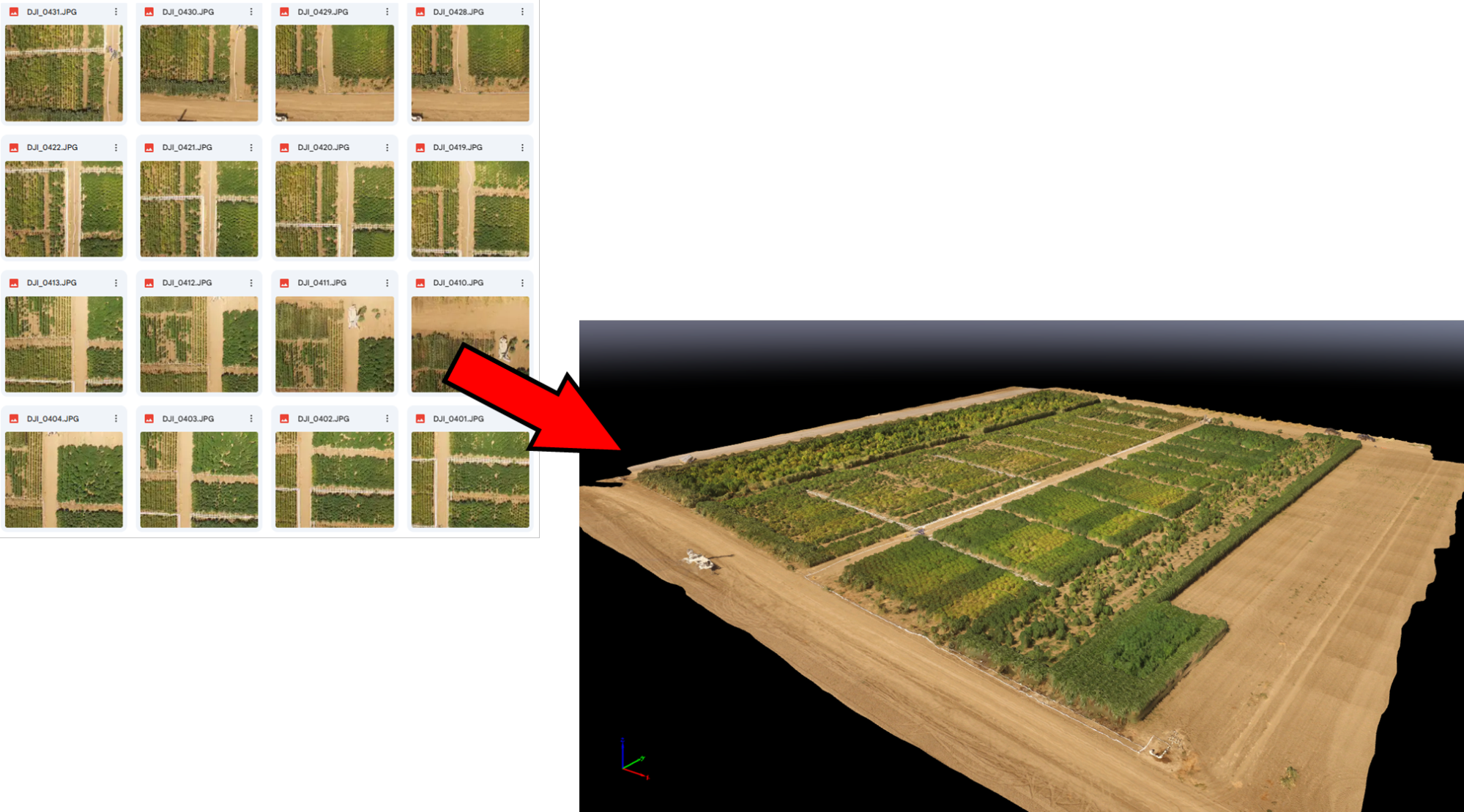
Wow. Pretty cool. And easy to use. Let’s jump into it.
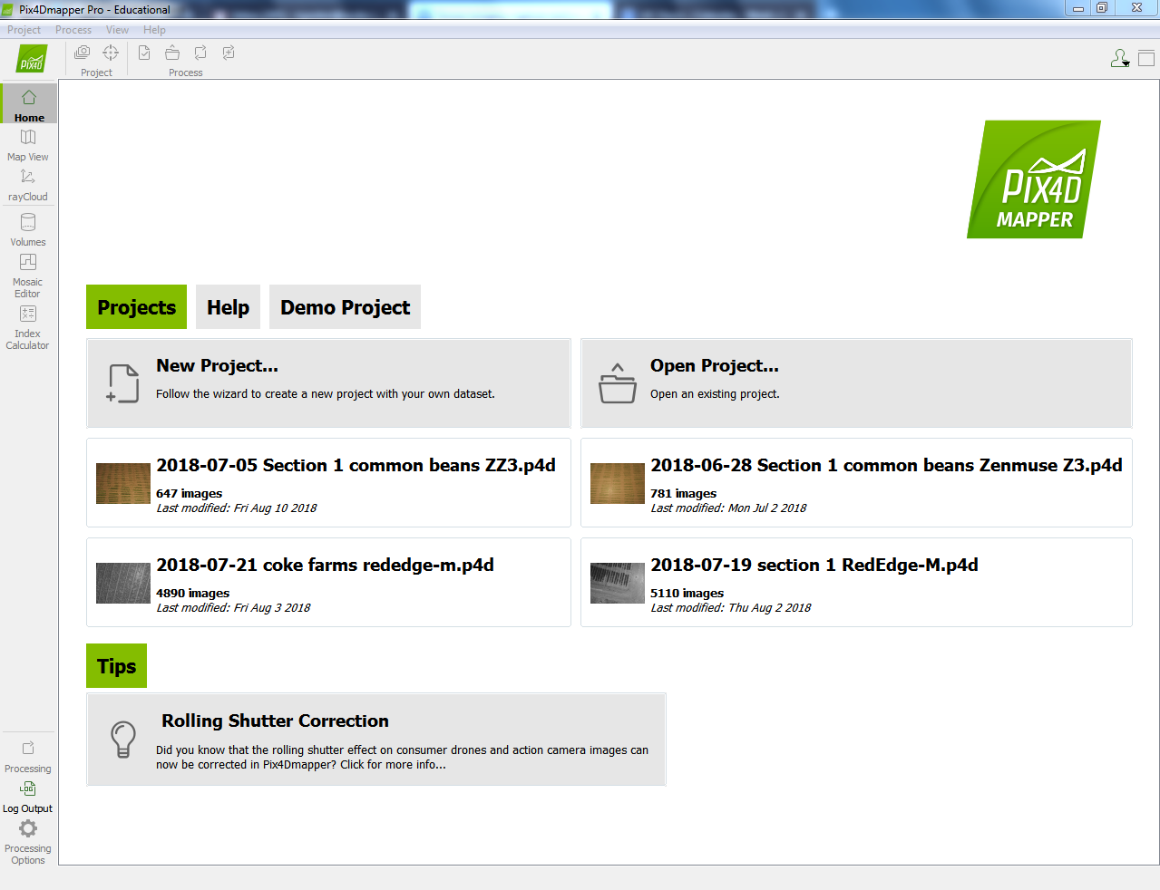
- Open Pix4Dmapper.
- Click “New Project”
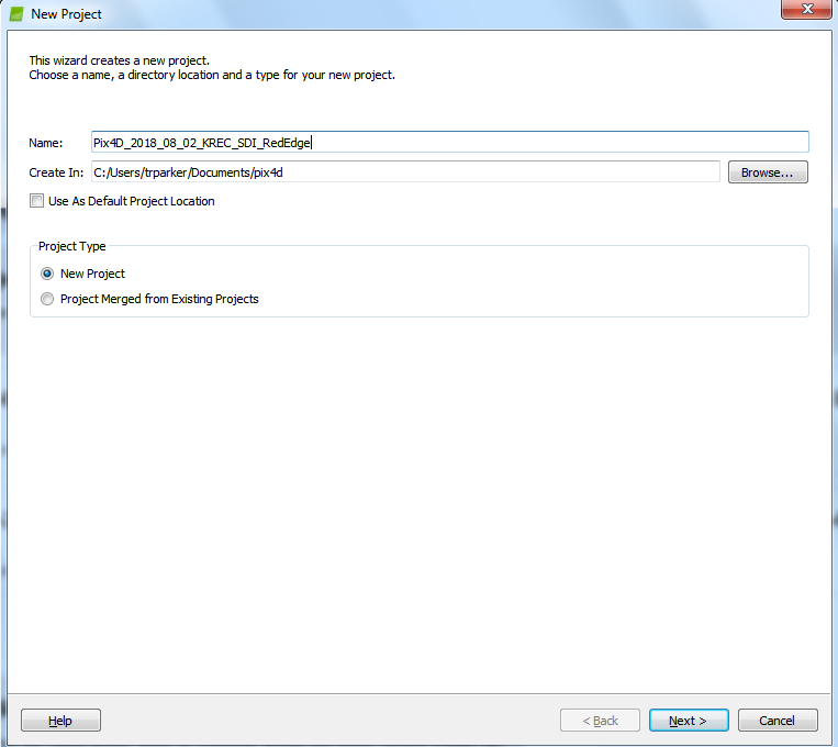
- Name the project. I often use the Year-Month-Day-Info format so things are organized chronologically.
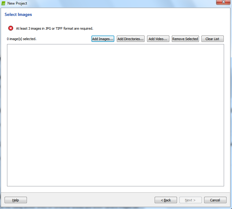
- Click “Add images”
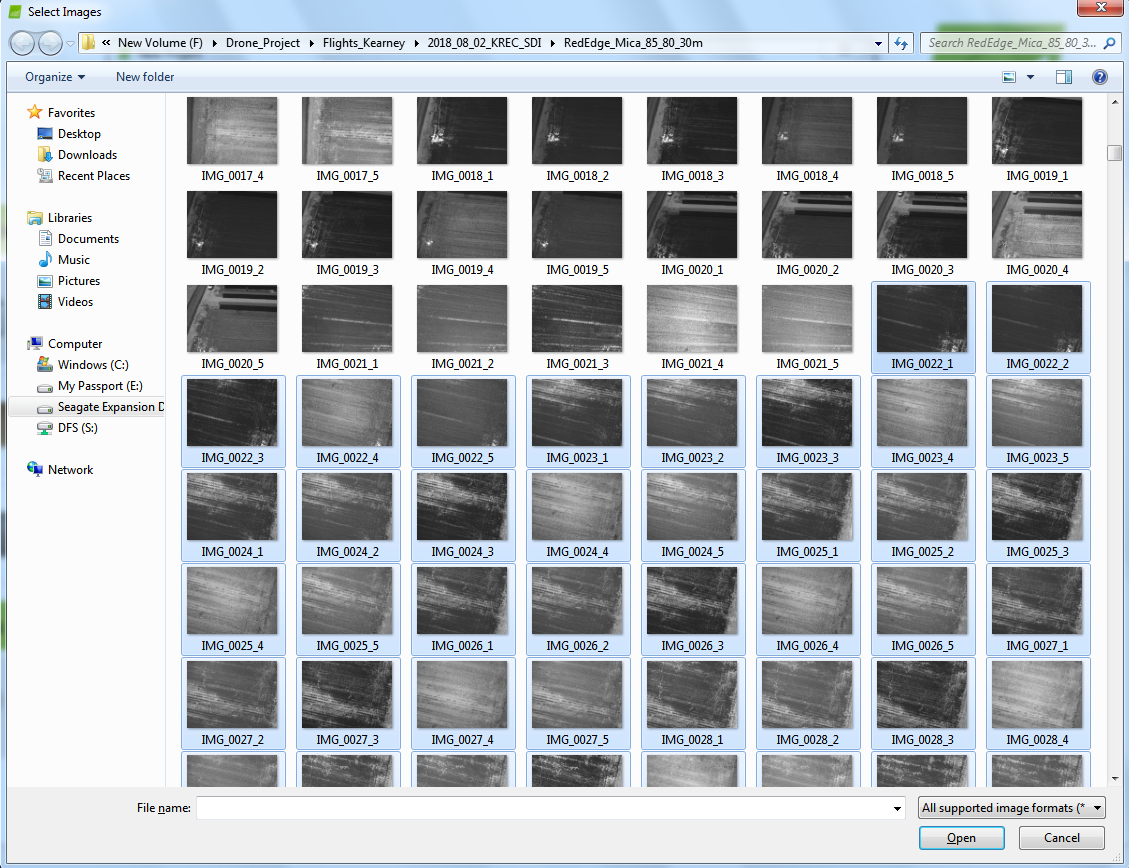
- Navigate to the folder of interest, and select images (often just Ctrl+A). Click “Open.”
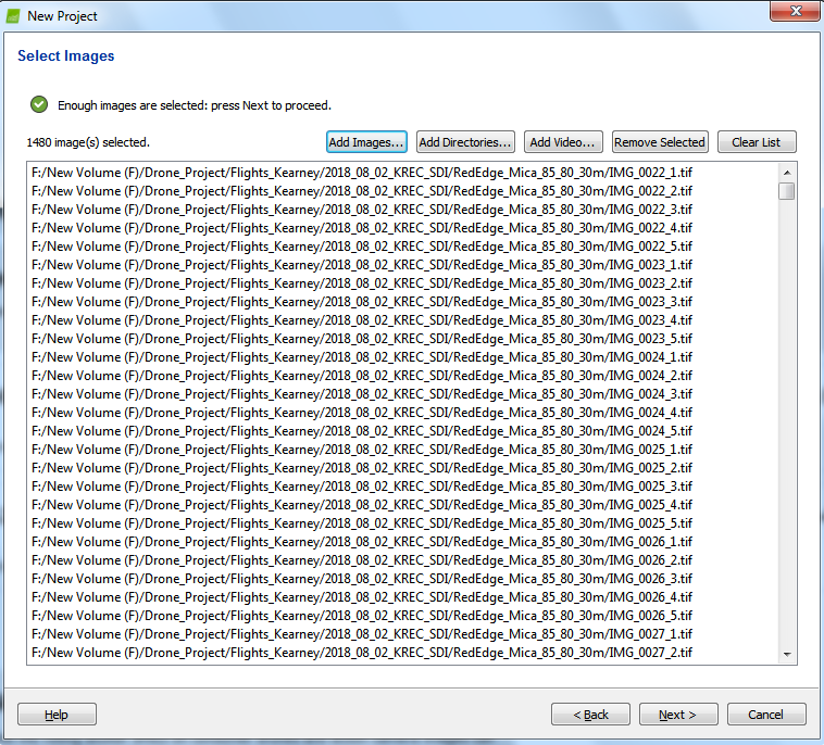
- Click “Next.”
- Check the number of geolocated images in the next pane. It would be unusual for any to not be geolocated, but if so, you could consider deleting. Click “Next.”
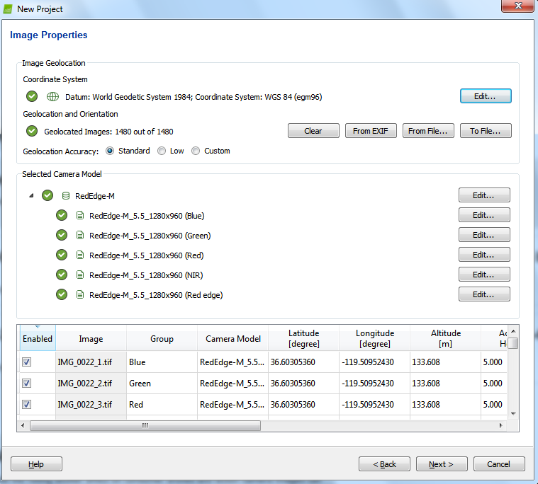
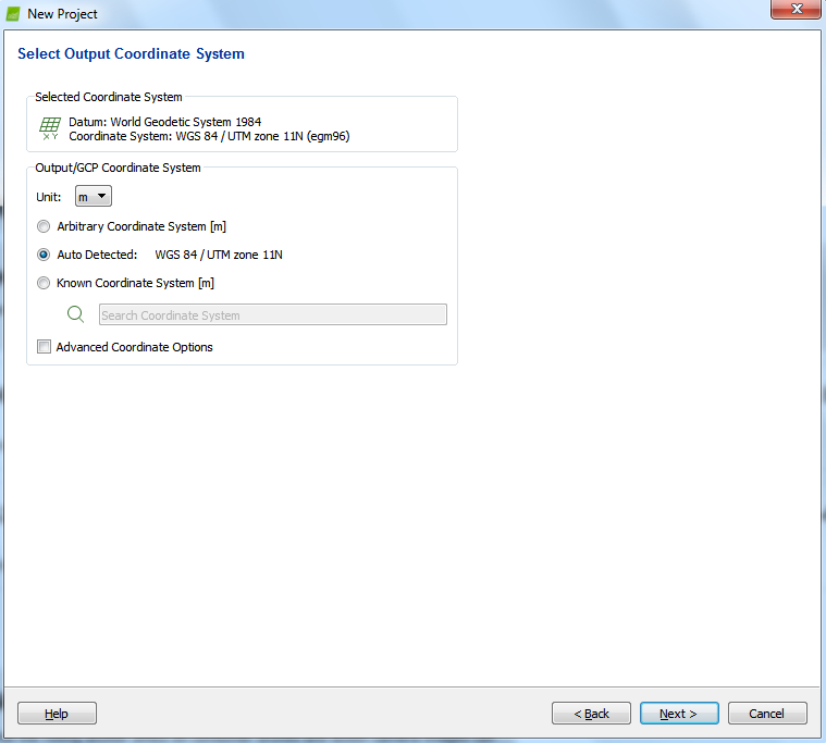
- Coordinate system info. Click “Next.”
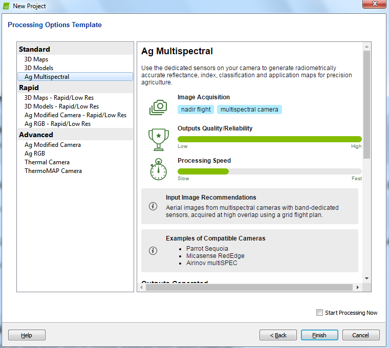
- Select the best processing option for your imagery type and needs. For multispectral cameras, choose “Ag multispectral.” For RGB cameras, I almost exclusively use “3D Maps”, and for thermal (Zenmuse XT-R) I use “Thermal Camera”. Information is provided for each on the right side. Do NOT click “Start Processing Now” at the bottom right. Click “Finish.”
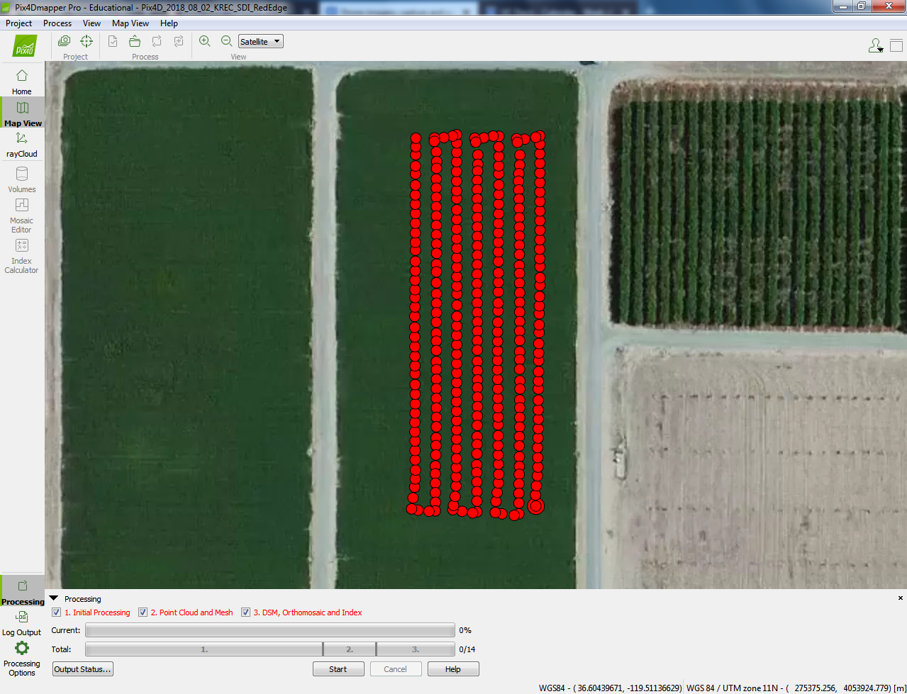
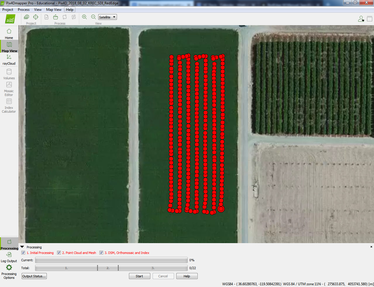
- You will now see a map with the locations of your image geotag positions. Click “Processing Options” at the bottom left.
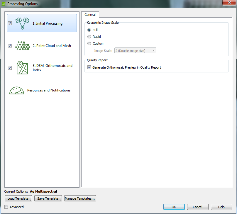
- In “1. Initial Processing” nothing usually needs to be adjusted. Click “2. Point Cloud and Mesh.”
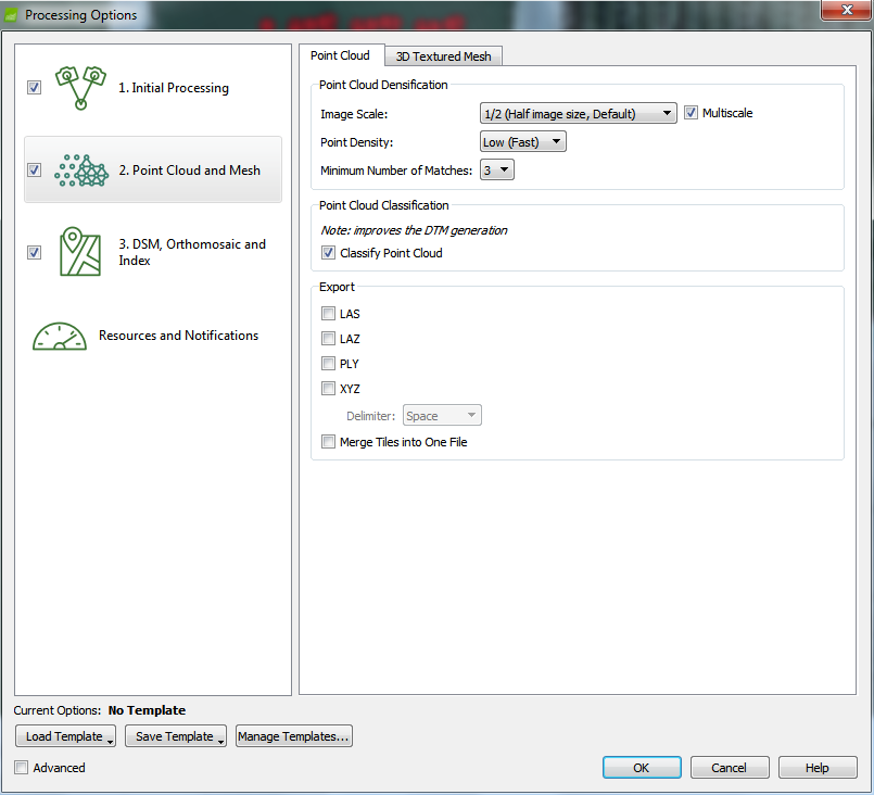
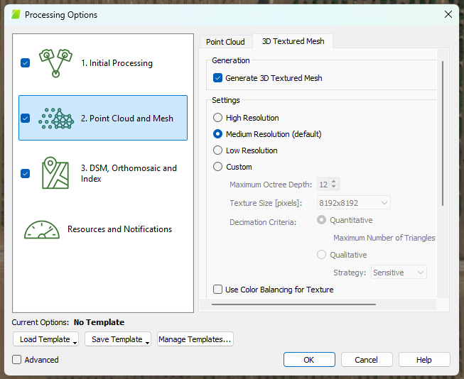
- If understanding the 3-dimensionality of your plots (i.e. canopy height and volume) is a priority, click “Classify Point Cloud.”
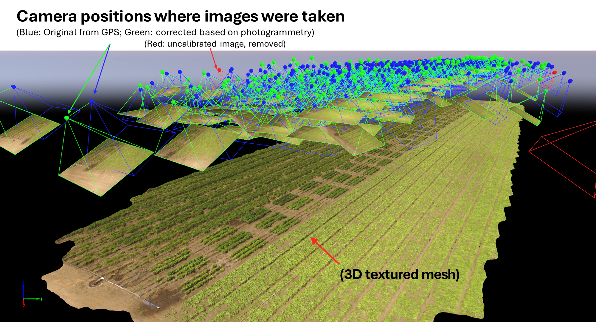
- Click the “3D Textured Mesh” tab at the top and make sure the box for “Generate 3D Textured Mesh” is checked. I mostly use these for display, but they are super beautiful 3D representations of your field. The next step is related to this idea…

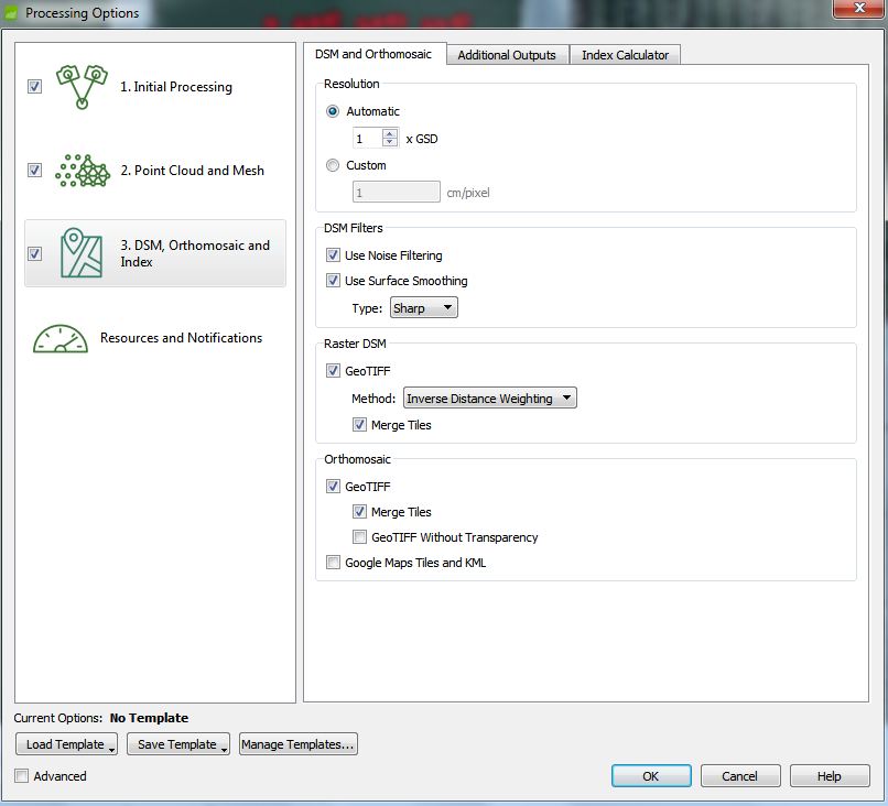
- On the left, click “3. DSM, Orthomosaic, and Index”. In the Raster DSM section, check the boxes for “Geotiff” and “Merge Tiles”. This will make it generate a raster digital surface model of your field… a 3D representation of the area, based on the geometry of features between images. For example, in a set of images from an orchard, the tops of trees will have different angles between images than if those same leaves were at ground level. This kind of thing is called “structure from motion photogrammetry”. It is super cool stuff.
- For RGB imagery, I would check the boxes for “GeoTIFF” and
“Merge Tiles” in the Orthomosaic section as well. These will give you a beautiful
representation of your field. The orthomosaics are less important for multispectral imagery, where
we will focus on the “Index Calculator” tab...
- Go to the “Additional Outputs” tab. Consider checking the box for “Geotiff” in the Raster DTM section. This is useful for comparing plant heights with predicted soil elevation.

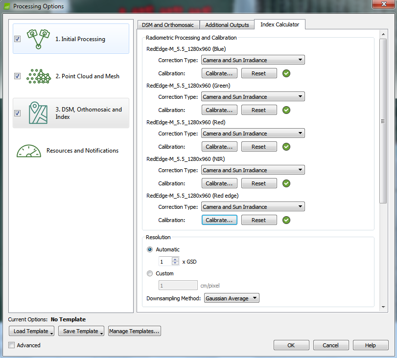
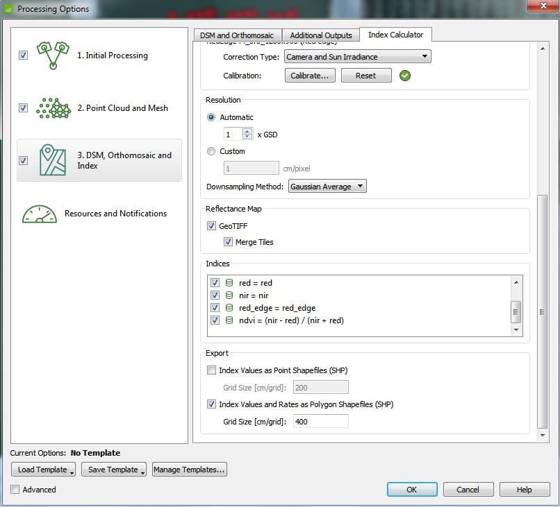
- Click the “Index Calculator” tab. For multispectral imagery, in
the section for Radiometric Processing and Calibration, these should be automatically read-in based
on the QR code. If the calibrations are set properly, you should see a green check mark. If these
are all green check marks (as shown below), skip the next step and go straight to section
19.
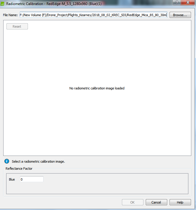
- If calibrations were not read in properly for one or more images, then you will see a small yellow exclamation point , and you will have to manually calibrate:
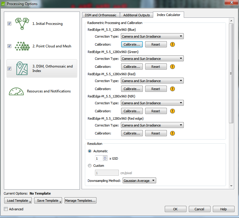
- Click “Calibrate” for these:
- In the new window, click “Browse” for a calibration image. For the RedEdge, the image numbers are ordered in the following way:
1: Blue
2: Green
3: Red
4: NIR
5: Red edge
This means that an image named “IMG_0003_2” will correspond to the green wavelength, because the FINAL number is 2.
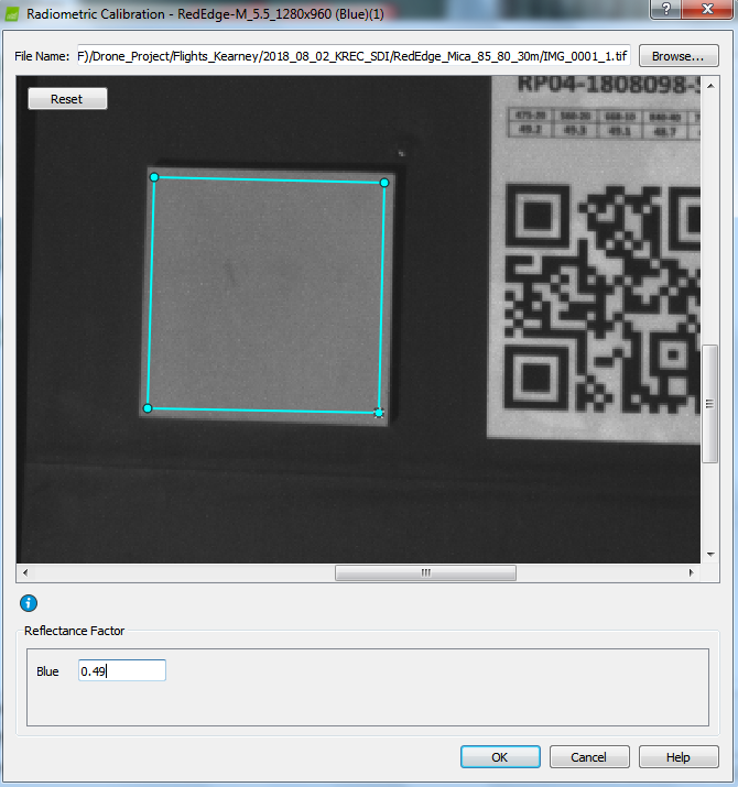
- After selecting your image, you can use your mouse to zoom in on the calibration panel. To draw your area of interest, left click three of the corners, and then right click the fourth and final corner. Right clicking will allow you to finish the shape. You will have to plug in a reflectance factor at the bottom, which will be specified by the manufacturer. Click “OK.”
- Repeat the process for the other wavelengths. You should have green
check marks next to all the bands.
- Scroll down. Check the box for “Merge tiles” in the Reflectance
Map section. Check the boxes for indices at all the other wavelengths. Click “OK.”
- The project is ready to begin. If you do not plan on adding ground control
points, you can hit “Start.” Ground control points can be added in Pix4d (or later in QGIS)
to increase the location accuracy. To use them here, uncheck the boxes for steps 2. and 3, then hit
“Start” . You will be prompted to add them later. After adding them, you will only need
to run steps 2 and 3, so you would un-check box 1 (“Initial Processing”) to not
over-write those results, then check boxes for steps 2 and 3, and hit
“Start”.
- After step 1 of the processing is completed, you will get a Quality report. Check it out! Usually, when things go well, I just skim it. If there were major issues in the processing, which is relatively uncommon, you will see that certain images might have been deactivated and shown in red. Sometimes you But this is uncommon.
- When the full processing is completed, check out your results. Try clicking the option for “3D Textured Mesh” and unselect “Tie Points”. Try activating and deactivating the other layer options too, why not:
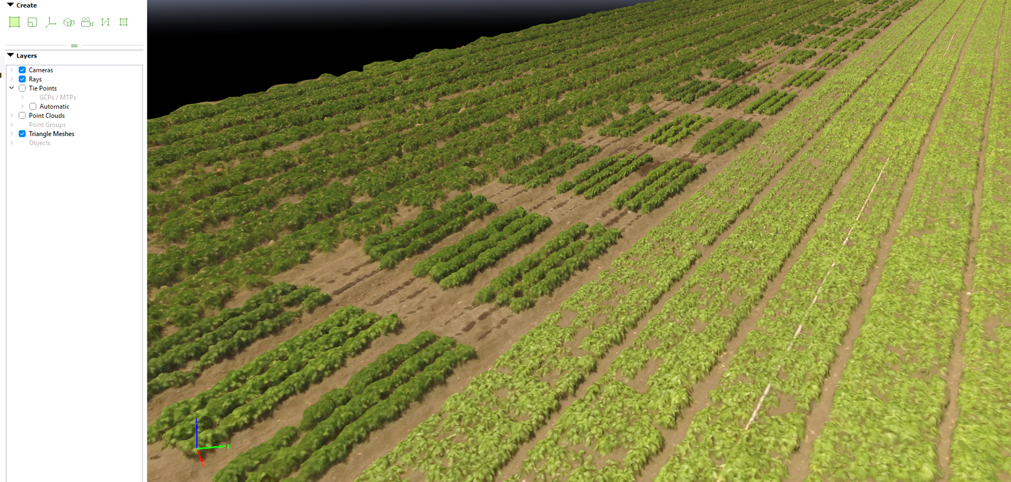
- Hold Shift and scroll with the mouse, then Ctrl and scroll. What do you think?
- Your results (by default) will be stored in
Documents/pix4d/PROJECT_NAME/. They will be divided into several folders. I tend to use the results
in the 3_dsm_ortho and 4_index folder the most. I typically delete any of the “tiles”
files.
- Files can be dragged and dropped into QGIS for visualization. More info on that in the next lessons!